

Sample Size for Carbon Project Surveys: How Many Households Are Enough?
This question gets answered badly more often than almost anything else in project design.
Someone proposes 5% of households. Someone else says 400 is a good number. A third person suggests 10% because it sounds thorough. All three are guessing, and the guess is usually discovered at verification, when a validation body asks how the sample size was derived and the honest answer is “it felt reasonable.”
The actual answer is neither arbitrary nor especially complicated. It’s also counterintuitive in one important way, which is where most of the confusion comes from.
The counterintuitive part
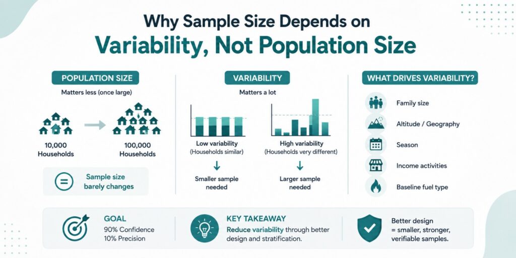
Sample size is driven mainly by how much your data varies, not by how many households you have.
This surprises people. The instinct is that a project with 100,000 households needs a much bigger sample than one with 10,000. In practice, once your population is reasonably large, the required sample barely moves. Going from 10,000 households to 100,000 might add very little to the sample you need.
What does move it, dramatically, is variability. If every household in your project burns roughly the same amount of firewood, you need surprisingly few observations to estimate the average confidently. If consumption ranges from 1 kg a day to 12 kg depending on family size, altitude, season and whether they run a small tea shop from the front room, you need a lot more.
This has a direct consequence for project design that most people miss: you can reduce your sample size by reducing variability, not just by surveying more. More on that below.
What the registries actually require
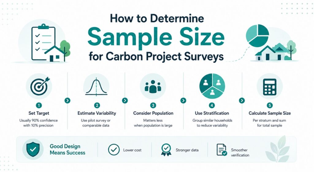
Most carbon crediting programmes specify sampling requirements in terms of confidence and precision, commonly expressed as 90/10 — 90% confidence with a 10% relative margin of error on the parameter you’re estimating.
In plain terms: if you repeated the survey many times, 90% of your estimates should land within 10% of the true value.
Some methodologies and parameters require tighter precision. Some allow different targets for different parameters within the same project. Check what your specific methodology requires before you design anything — this is not a place for a general rule of thumb, and the requirement sometimes changes between methodology versions.
The three inputs you need
To calculate a sample size properly, you need:
1. Your confidence and precision target — from your methodology. Usually 90/10.
2. An estimate of variability — expressed as the coefficient of variation, which is just the standard deviation divided by the mean. This is the input people don’t have, and it’s the one that matters most.
3. Your population size — which, as established, matters less than you’d expect for large populations.
The formula itself is specified in registry sampling standards and is not the hard part. Any competent statistician or a decent MRV partner can run it. The hard part is input two.
Where the variability estimate comes from
You have three options, in descending order of reliability.
A pilot survey. Survey 40–60 households across your project geography, calculate the coefficient of variation from the real data, and use it. This costs money and time upfront, and it is almost always worth it. A pilot that costs a few lakh can prevent a sample design that costs many times that in either wasted surveys or a failed verification.
Data from a comparable project. Same region, same intervention, similar household profile. Usable, but adjust upward for uncertainty — your population is not their population.
A conservative assumption. Pick a high coefficient of variation, accept a larger sample, and move on. Safe, expensive, and the default when nobody planned ahead.
The trap here is circular: to know your sample size you need to know your variability, and to know your variability you need data. The pilot breaks the circle. Skipping it means guessing, and guessing conservatively is the only responsible way to guess — which means paying for a bigger sample than you probably needed.
Stratification: the lever most projects don’t pull
This is where real savings live.
If your project spans three states with very different fuel use patterns, treating it as one population means your variability estimate absorbs all that between-state difference. Your sample size balloons to accommodate it.
Split the population into strata that are internally similar — by state, by altitude band, by household size, by baseline fuel type — and calculate a sample for each. Within a stratum, variability is lower. The total sample across strata is often meaningfully smaller than the single-population sample, and the estimate is better.
Stratification also protects you from a specific failure: a simple random sample can, by chance, under-represent a subgroup that behaves very differently. That’s the kind of thing a verifier notices.
The cost is design complexity and a slightly harder field operation. It’s usually worth it.
Five ways sample designs fail in practice
The calculation is rarely the problem. Execution is.
1. Replacement rules that were never written down. A selected household is locked, migrated, or refuses. Field teams substitute the neighbour. Do this systematically and you’ve quietly replaced a random sample with a convenience sample of whoever was home — which skews toward households with someone free during the day.
Define replacement rules in advance. Document every substitution.
2. Non-response that never gets recorded. If you don’t track refusals and unavailability, you can’t demonstrate your sample is still representative. Verifiers ask.
3. Attrition across monitoring cycles. Your sample was valid in year one. By year four, households have migrated, dropped out, or become unreachable. If your effective sample has quietly fallen below the required size, your later credits are on shakier ground than your earlier ones.
Design for attrition from the start. Over-sample modestly if your methodology permits.
4. Clustering for convenience. Sampling three villages instead of thirty because it’s cheaper does reduce cost. It also changes your effective sample size, because households within a village resemble each other. If you cluster, account for it in the calculation. Many projects cluster and don’t.
5. Post-hoc sample size. Surveying whatever was affordable and back-fitting a justification. This is the one verifiers are best at spotting, because the arithmetic doesn’t reconcile.
A practical sequence
If you’re designing this from scratch:
- Read your methodology’s sampling requirement. Note the confidence and precision target and any parameter-specific rules.
- Decide your strata before anything else. Geography, baseline fuel, household size — whatever genuinely drives variation in your context.
- Run a pilot across strata. 40–60 households is usually enough to estimate variability.
- Calculate per stratum, then sum.
- Add for attrition across the crediting period.
- Write down replacement and non-response rules before fieldwork begins.
- Document everything — the derivation, the pilot data, the assumptions. This document is what a verifier will ask for.
The honest bottom line
A defensible sample is smaller than most people fear and larger than most budgets initially allow.
The failure mode isn’t usually a sample that’s too small. It’s a sample whose size nobody can justify, drawn by a method nobody wrote down, degraded by substitutions nobody recorded. That fails verification even when the number itself was fine.
Spend the money on the pilot and the documentation. It’s cheaper than surveying households you didn’t need, and considerably cheaper than a verification query eighteen months after your field team has moved on.
Anaxee’s Climate Command Centre designs and executes sampling for Indian carbon projects — pilot surveys, stratified designs, documented replacement protocols and back-checked field collection across 540+ districts and 11,000+ pincodes. If you’re designing a monitoring sample, talk to our team.